Optimizing Spatial Subdivisions in Practice
As outlined in the earlier Spatial Subdivisions post, not all spatial data structures are equal. But how well do our tweaks to the classic quadtree/octree algorithm hold up in practice?
In the case of 3D Tiles for streaming to Cesium, we evaluate tilesets using a couple of questions including:
- How deep is the tileset? Tiles deeper in the tileset take longer to load and display, which can be a problem if a user is zooming into a high detail area.
- How "balanced" is the tileset? In an unbalanced tree, high detail geometry can be slower to load in some areas than in others.
- How even is the data distribution across tiles? Tiles that contain too many points or triangles take too long to download and draw, but too many "small" tiles limits network and GPU efficiency.
Here's a drone capture of a church in Lancaster, Pennsylvania converted to a 3D model using Bentley ContextCapture, and tiled for streaming to Cesium using our upcoming tiling pipeline in Cesium Composer. The model straight out of ContextCapture consisted of ~1.7 million triangles and 192 megapixels of texture data. Since this is a photogrammetry model, the triangles are mostly the same size and are fairly evenly distributed; this isn't a model where a very small area is extremely expensive, which is the type of model that tends to show a lot of problems for the traditional octree algorithm.
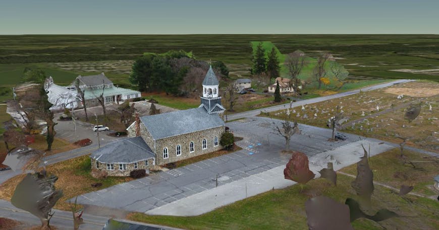
Church in Lancaster
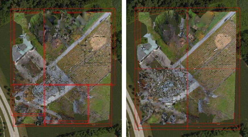
We tiled this model twice, once using a traditional uniform octree method and once using an optimized non-uniform algorithm based on the concepts described in the previous Spatial Subdivision blog post. Below, the optimized octree is on the left, while the "traditional" octree is on the right. The bounding volumes for each look a little different:
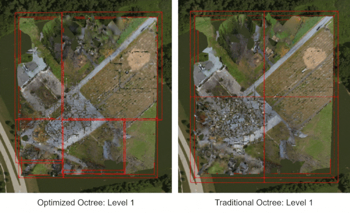
The uniform octree should look familiar to readers who typically work with 2D quadrees, such as for terrain or imagery - it's just the same algorithm extended to 3D.
The optimized non-uniform octree, on the other hand, looks a lot more chaotic, with bounding boxes of all kinds of sizes. However, note that the few large bounding boxes tend to cover the surrounding grounds, while most of the smaller bounding boxes cover the church building itself. This is the most triangle-dense part of the mesh so the octree adaptively has a higher concentration of tiles in this area.
Drawing out the hierarchy as a tree gives a better idea of the difference between the two tilesets. Leaf tiles containing original resolution geometry and textures are marked in green.
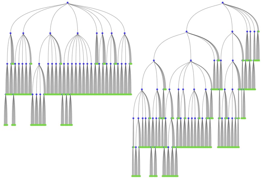
Left) Optimized non-uniform octree. Right) Traditional uniform octree.
We can see from these diagrams that the optimized octree is both better balanced and shallower than the traditional version. Going back to the bounding volumes, we see that the optimized octree attempts to divide the church building across different tiles from the very first level of subdivision, leading to better balance.
Bounding volumes at level 1. Left) Optimized non-uniform octree. Right) Traditional uniform octree.
Finally, how does data distribution look? Here's a coarse histogram for each octree's file sizes, which approximates data distribution:


The optimized octree shows a lower count of tiles smaller than 200 KB, which means the optimized tileset will render better using GPUs that can easily draw more than 200 KB of triangles and textures in the time allotted to one frame.
Finally, since the distribution for tiles greater than 200 KB is similar between the two methods, the overall tile count is less in the optimized tileset. Here's a level-by-level comparison of tile counts:
| level | optimized | traditional |
|---|---|---|
| 0 | 1 | 1 |
| 1 | 8 | 8 |
| 2 | 64 | 39 |
| 3 | 234 | 70 |
| 4 | 69 | 87 |
| 5 | 0 | 175 |
| 6 | 0 | 61 |
| total tiles | 376 | 454 |
As always, the best way to verify what we've made is to tile more 3D models. Feel free to ping me at gary@cesium.com or tweet to @CesiumJS if you have any massive models that you want to stream to Cesium.