Optimizing Subdivisions in Spatial Data Structures
Spatial Subdivision techniques are essential in almost all areas of computer graphics, and are very popular in both 2D and 3D digital cartography. In 3D Tiles, they simplify rendering by grouping large amounts of geometry into tiles that are likely to be visible at the same time and provide a hierarchy so not every tile has to be checked when determining what should be streamed and rendered.
Spatial data structures form the backbone of 3D Tiles. They all have one thing in common: child tiles have geometry that fit within their parent tile’s bounding volume. Here’s a quick algorithm for building a 2D quadtree that conforms to this rule:
- start with a bounding box that encompasses all the geometry
- split that bounding box evenly into child quads
- for each child quad, repeat until you have n triangles per quad.
Here are recordings of an interactive demo built on this algorithm. Areas with darker blue are “deeper” in the tree.
Left click to add points, left click on a point to remove it
Hold left click to wipe the tree and immediately scatter some random points
A standard quadtree is a wonderful way to partition relatively uniform data, such as the random points in this demo. It’s also why quadtrees work very well for raster data, which take up the entire space. However, when geometry is relatively sparse, the tree easily becomes inefficient. Take this quadtree, for example:
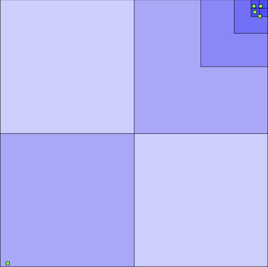
Traditional quadtree with sparse data
The quadtree is pretty unbalanced, going deeper in the top right than in the bottom left. If we had simplified geometry in each non-leaf tile for Hierarchical Level Of Detail (HLOD), we would have a chain of simplifications to go through before reaching the original geometry in the top right. In addition, the tiles in the top right quadrant mostly encompass the same thing, with useful distinction only on the smallest tiles - so each simplification in that chain would essentially be of the same thing, removing one of the advantages of HLOD. Finally, there are a lot of tiles that cover much more area than their actual geometry, which makes frustum culling much less effective.
In these cases, we benefit from picking each tile’s bounding box and splitting the bounding box into child quads differently. For example, one easy change is to use an initial bounding box that only encompasses the given geometry and then pick how we subdivide the children based on density. Performing both techniques recursively leads to much better results. Switching from the traditional quadtree to our density-based non-uniform quadtree on the same set of points produces this:
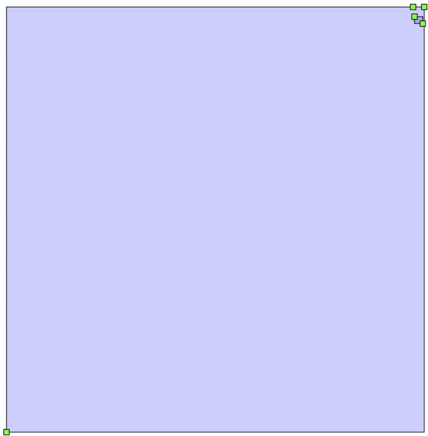
Sparse data using Cesium's density-based non-uniform quadtree
If we were to draw out the tileset for the two subdivisions, they might look something like this:
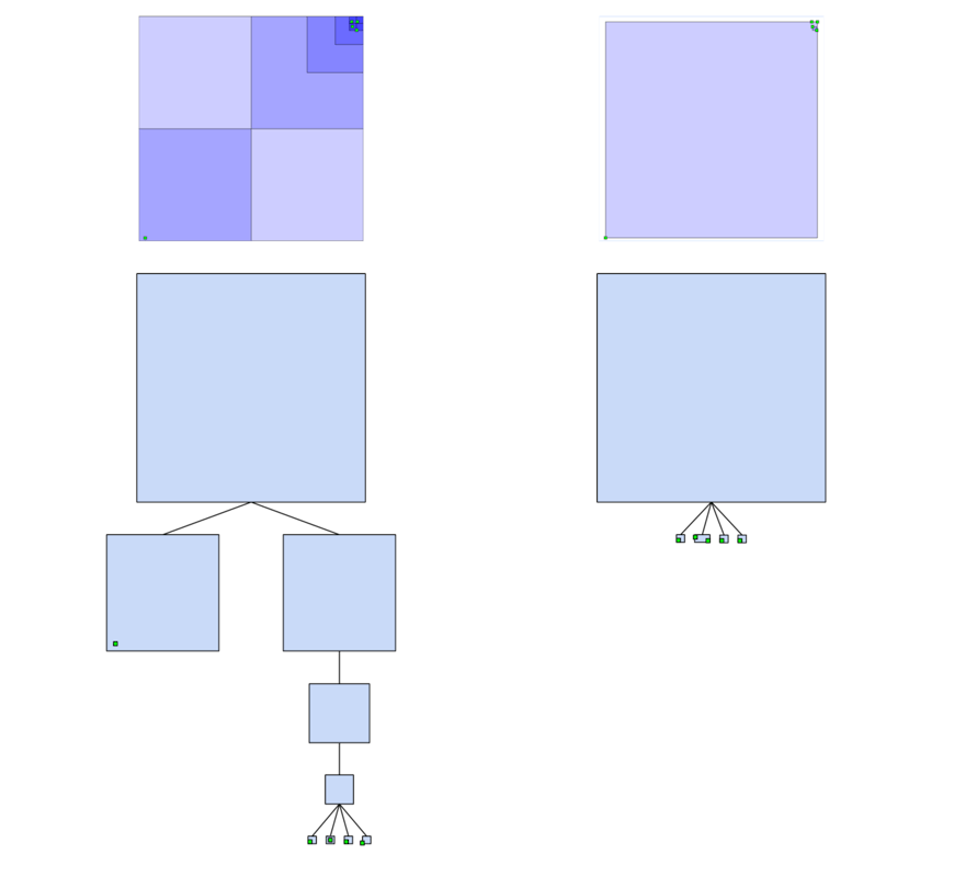
The non-uniform tileset on the right has a more balanced, shallower tree with tighter bounding volumes, all of which lead to better rendering efficiency.
Other algorithms may be even better suited for getting around the efficiency problems of uniform quadtrees. A k-d tree, for example, can be extremely well balanced if constructed roughly as follows:
- compute the “center” along one axis of all geometry in a region
- divide the region into two child regions based on that center
- repeat for each child region, rotating the axis for subdivision
Clicking to add points to a k-d tree
Wiping and distributing random points in a k-d tree
Since a k-d tree always splits the geometry in a region in half, the resulting tree can be extremely well balanced, depending on the criterion for “center”. However, since each split can only produce two new tiles instead of the quadtree’s 4 or an octree’s 8, k-d trees tend to become very deep for large datasets.
The big takeaway here is that there is rarely a perfect “one size fits all” spatial data structure algorithm. Fortunately, the flexibility written into the 3D Tiles specification allows users to implement virtually any 2D or 3D spatial data structure - users can even mix and match subdivision strategies within a tileset to suit different types of data.